🤖 拿上你的酒,是时候揭开 ML 和 NLP 的神秘面纱了🍷
这是一个正确的预测!🎉

在本教程中,您将学习如何使用 ML 根据文本描述预测葡萄酒的价格、积分和品种。
我们将使用SciKit Learn库处理葡萄酒描述文本,创建一个词袋逻辑回归多分类模型。如果您还没理解,那么您来对地方了!如果您理解了,请继续阅读,因为葡萄酒。
配置您的 ML 开发环境
有两个选项:云或本地。
Azure 云设置 - 使用 Azure 机器学习工作区与集成的云 Notebook 虚拟机。工作区提供了丰富的功能,我强烈推荐它。
- 如果您还没有 Azure 帐户,请创建一个免费的Azure 帐户。
- 按照创建工作区教程中的“创建笔记本虚拟机”步骤进行操作
- 从 Notebook VM 导航中单击“Jupyter Lab”
- 然后在终端中运行以下命令从 GitHub 克隆笔记本。

#CTRL+SHIFT+V to paste
curl https://raw.githubusercontent.com/cassieview/intro-nlp-wine-reviews/master/winereview-nlp.ipynb --output winereview-nlp.ipynb
本地设置
- 下载 Jupyter笔记本
- 下载 Anaconda
- 运行 Jupyter 笔记本
一旦您设置了上述环境配置之一,就可以开始构建了!
导入包和数据
如果出现“无模块名称”错误,请使用命令进行安装!pip install wordcloud。 将其替换wordcloud为错误消息中的模块名称。
#This package need to be installed first
!pip install wordcloud
import pandas as pd
import numpy as np
import matplotlib.pyplot as plt
import seaborn as sns
import math
from sklearn.model_selection import train_test_split
from sklearn.metrics import precision_recall_curve
from sklearn.linear_model import LogisticRegression
from sklearn.feature_extraction.text import CountVectorizer
from joblib import dump, load
我们需要数据!我使用了在 Kaggle 上找到的数据集。Kaggle 是一个数据科学家的在线社区。您可以从 GitHub 仓库或 Kaggle 下载数据集。

将数据导入为Pandas DataFrame
#File path to the csv file
csv_file = "https://raw.githubusercontent.com/cassieview/intro-nlp-wine-reviews/master/dataset/winemag-review.csv"

# Read csv file into dataframe
df = pd.read_csv(csv_file)

# Print first 5 rows in the dataframe
df.head()

可视化数据
一旦我们有了数据,就该分析它并进行一些特征选择和工程了。我们将使用Seaborn将数据可视化。这将使我们能够看到不同数据点之间是否存在很强的相关性,并帮助我们回答有关数据的问题。由于我们最初的问题是关于预测price,points或者variety从我们description已经知道我们的特征将是description,我们的标签将是price,points或variety。特征是我们用来进行预测的数据,标签是我们要预测的内容。每个标签将是一个单独的模型,因此如果您选择构建所有三个预测模型,则总共会有三个模型。
为了好玩,让我们问一些有关数据的问题,并通过用 Seaborn 绘制图表来回答它们。
价格和积分之间有关联吗?
sns.barplot(x = 'points', y = 'price', data = df)

sns.boxplot(x = 'points', y = 'price', data = df)

是否有一位葡萄酒评论家给出的评分比其他评论家更高?
sns.catplot(x = 'points', y = 'taster_name', data = df)

让我们看一下description文本的词云
from wordcloud import WordCloud, STOPWORDS
import matplotlib.pyplot as plt
text = df.description.values
wordcloud = WordCloud(
    width = 3000,
    height = 2000,
    background_color = 'black',
    stopwords = STOPWORDS).generate(str(text))
fig = plt.figure(
    figsize = (40, 30),
    facecolor = 'k',
    edgecolor = 'k')
plt.imshow(wordcloud, interpolation = 'bilinear')
plt.axis('off')
plt.tight_layout(pad=0)
plt.show()
我喜欢把这个词云看作是品尝葡萄酒时使用的描述性词语的备忘单,让自己听起来像个葡萄酒专家😃
通过绘制这些数据图表,您还可以提出和回答哪些其他问题?
为标签创建计算列
这将对葡萄酒评论家评测的葡萄酒的价格点或葡萄品种进行多重分类。目前,我们的点数和价格是数字特征。这需要更新为文本特征类别,为此,我们将创建几个函数,根据点数和价格列中的值生成计算列,用作我们的标签。
创建列,根据分数值将分数分为“差”、“还行”、“好”和“优秀”。下面是一个根据分数值quality返回字符串的函数。quality
def getQuality(points):
    if(points <= 85):
        return 'bad'
    elif(points<=90 ):
        return 'ok'
    elif(points<=95):
        return 'good'
    elif(points<=100):
        return 'great'
    else:
        return 'If this gets hit, we did something wrong!'
接下来将函数应用到数据框的点列并添加一个名为的新列quality。
df['quality'] = df['points'].apply(getQuality)
像我们上面所做的那样,将新列与价格列进行可视化。
sns.catplot(x = 'quality', y = 'price', data = df)

sns.barplot(x = 'quality', y = 'price', data = df)

对于包含 NaN 的列,根据 、 、 和1-30的31-50价格51-100列创建 priceRange 列。以下函数用于根据价格值返回字符串 priceRange。Above 1000
def getPriceRange(price):
    if(price <= 30):
        return '1-30'
    elif(price<=50):
        return '31-50'
    elif(price<=100):
        return '51-100'
    elif(math.isnan(price)):
        return '0'
    else:
        return 'Above 100'
将函数应用于数据框的点列并添加一个名为的新列priceRange。
df['priceRange'] = df['price'].apply(getPriceRange)
打印每个指定 priceRange 的总数,以查看标签的分布情况
df.groupby(df['priceRange']).size()
Output: priceRange
        0             8996
        1-30         73455
        31-50        27746
        51-100       16408
        Above 100     3366
        dtype: int64
我们现在有了用于预测质量、价格范围和葡萄品种的模型标签。
使用库 SciKit 处理描述文本,学习使用CountVectorizer功能创建词袋。
文档对 CountVectorizer 的解释非常到位。我建议大家通读一遍,以便全面了解其工作原理,不过这里我还是会先介绍一些基础知识。
从高层次上讲,CountVectorizer 会获取描述的文本,删除停用词(例如“the”、“a”、“an”、“in”),对单词进行标记化,然后创建一个表示描述的数字向量。文本描述现在以数字形式表示,只包含我们关心的单词,可以由计算机处理以训练模型。记住,计算机理解数字,而单词也可以表示为数字,因此计算机可以“理解”。
这是一个单词如何转化为数字的例子。我们将通过数据集中的示例来更详细地讲解这一点。

在我们深入了解 CountVectorizer 的代码和功能之前,我想列出一些术语,并指出 CountVectorizer不会为您进行词形还原或词干提取。
- 停用词:停用词可以是特定语言中有意义的单词。例如,在英语中,“a”、“and”、“is”和“the”等词会被排除在全文索引之外,因为它们对搜索毫无用处。停用词也可以是没有语言含义的标记。
-
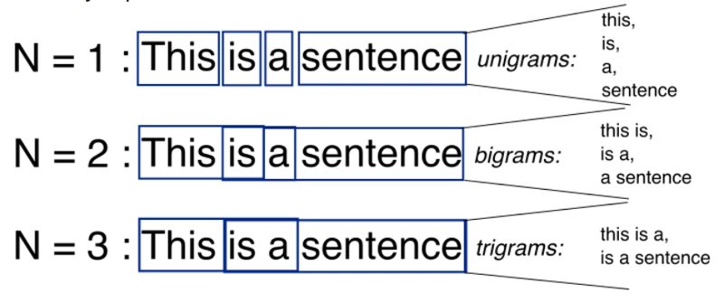
N-Gram:一种文本数据的特征提取方案:任何由 N 个单词组成的序列都会变成一个特征值。
-
词形还原:将多个相关词转换为单一的规范形式(“fruity”、“fruitiness”和“fruits”都将转换为“fruit”)
-
词干提取:与词形还原类似,但更具侵略性,可能会使词语变得碎片化。

让我们看一下如何使用 CountVectorizer。
这些是您可以在 CountVectorizer 中设置的所有属性。其中许多属性是默认的,或者如果设置了,则会覆盖 CountVectorizer 的其他部分。我们将保留大部分默认值,然后尝试更改其中一些,以获得更好的模型结果。
CountVectorizer(
  input='content', encoding='utf-8', decode_error='strict',
  strip_accents=None, lowercase=True, preprocessor=None, tokenizer=None,
  stop_words=None, token_pattern='(?u)\b\w\w+\b', ngram_range=(1, 1),
  analyzer='word', max_df=1.0, min_df=1, max_features=None,
  vocabulary=None, binary=False, dtype=<class 'numpy.int64'>
)
创建函数以从description特征中获取向量和矢量化器。
CountVectorizer 的不同配置已被注释掉,以便我们尝试不同的配置,并观察其对结果的影响。此外,这还能帮助我们通过一个描述,了解 CountVectorizer 中实际发生的情况。
def get_vector_feature_matrix(description):
    vectorizer = CountVectorizer(lowercase=True, stop_words="english", max_features=5)
    #vectorizer = CountVectorizer(lowercase=True, stop_words="english")
    #vectorizer = CountVectorizer(lowercase=True, stop_words="english",ngram_range=(1, 2), max_features=20)

    #vectorizer = CountVectorizer(lowercase=True, stop_words="english", tokenizer=stemming_tokenizer)
    vector = vectorizer.fit_transform(np.array(description))
    return vector, vectorizer
首次运行时,我们将使用以下配置。这意味着我们要将文本转换为小写,删除英文停用词,并且只使用 5 个单词作为特征标记。
vectorizer = CountVectorizer(lowercase=True, stop_words="english", max_features=5)
#Optional: remove any rows with NaN values.
#df = df.dropna()
接下来让我们调用我们的函数并传入数据框中的描述列。
这将返回vector和vectorizer。vectorizer我们将 应用于文本,以创建vector文本的数字表示,以便机器学习模型可以学习。
vector, vectorizer = get_vector_feature_matrix(df['description'])
如果我们打印矢量化器,我们可以看到它的当前默认参数。
print(vectorizer)
Output: CountVectorizer(analyzer='word', binary=False, decode_error='strict',
        dtype=<class 'numpy.int64'>, encoding='utf-8', input='content',
        lowercase=True, max_df=1.0, max_features=5, min_df=1,
        ngram_range=(1, 1), preprocessor=None, stop_words='english',
        strip_accents=None, token_pattern='(?u)\\b\\w\\w+\\b',
        tokenizer=None, vocabulary=None)
检查我们的变量和数据以了解这里发生的事情。
print(vectorizer.get_feature_names())
Output: ['aromas', 'flavors', 'fruit', 'palate', 'wine']
这里我们获取了向量化器的特征。因为我们告诉 CountVectorizer 有一个,max_feature = 5它会构建一个词汇表,该词汇表只考虑语料库中按词频排序的顶级特征词。这意味着我们的description向量在标记化时只会包含这些词,所有其他词都会被忽略。
打印出我们的第一个description和第一个vector来查看其表示。
print(vector.toarray()[0])
Output: [1 0 1 1 0]
df['description'].iloc[0]
Output: "_Aromas_ include tropical _fruit_, broom, brimstone and dried herb. The _palate_ isn't overly expressive, offering unripened apple, citrus and dried sage alongside brisk acidity."
表示语料库中第一个描述的[1 0 1 1 0]矢量化特征()的矢量数组( )。1 表示按矢量化特征的顺序存在,0 表示不存在。['aromas', 'flavors', 'fruit', 'palate', 'wine']
尝试一下向量和描述的不同索引。你会注意到,这里没有词形还原,所以像fruityand这样的词fruits会被忽略,因为只有fruit包含在向量中,而我们没有对描述进行词形还原以将它们转换为词根。
训练模型
更新该函数以便使用第二个矢量化器配置。
def get_vector_feature_matrix(description):
    #vectorizer = CountVectorizer(lowercase=True, stop_words="english", max_features=5)
    vectorizer = CountVectorizer(lowercase=True, stop_words="english", max_features=1000)
    #vectorizer = CountVectorizer(lowercase=True, stop_words="english",ngram_range=(1, 2), max_features=1000)
    #vectorizer = CountVectorizer(lowercase=True, stop_words="english", tokenizer=stemming_tokenizer)
    vector = vectorizer.fit_transform(np.array(description))
    return vector, vectorizer
并调用函数来更新矢量化器
vector, vectorizer = get_vector_feature_matrix(df['description'])
现在创建我们的特征矩阵。如果出现 MemoryError,请减少 CountVectorizer 中的 max_features 值。
features = vector.todense()
我们为三个不同的模型设置了三个不同的标签。接下来,我们先赋值标签变量,并quality首先使用标签。
label = df['quality']
#label = df['priceRange']
#label = df['variety']
我们已经创建了特征和标签变量。接下来我们需要拆分数据以进行训练和测试。
我们将使用 80% 的数据进行训练,20% 的数据进行测试。这将使我们能够从训练中获得准确率估计,以了解模型的运行情况。
X, y = features, label
X_train, X_test, y_train, y_test = train_test_split(X, y, test_size=0.2)
使用LogisticRegression算法训练模型并打印准确度。
lr = LogisticRegression(multi_class='ovr',solver='lbfgs')
model = lr.fit(X_train, y_train)

accuracy = model.score(X_test, y_test)
print ("Accuracy is {}".format(accuracy))
Output: "Accuracy is 0.7404885554914407"
这个准确度还算可以,但我相信还可以改进!在本教程中,我们称之为“足够好”,这是你构建的每个模型都需要做出的决定!
测试模型
当你选择一个候选模型时,应该始终在未见过的数据上进行测试。如果一个模型与其数据过度拟合,那么它在自身数据上的表现会很好,而在新数据上的表现会很差。这就是为什么在未见过的数据上进行测试非常重要。
我从葡萄酒杂志网站上抓取了这篇评论。这是一篇95分、售价60美元一瓶的葡萄酒评论。
test = "This comes from the producer's coolest estate near the town of Freestone. White pepper jumps from the glass alongside accents of lavender, rose and spice. Compelling in every way, it offers juicy raspberry fruit that's focused, pure and undeniably delicious."


x = vectorizer.transform(np.array([test]))
proba = model.predict_proba(x)
classes = model.classes_
resultdf = pd.DataFrame(data=proba, columns=classes)
resultdf

这是一个正确的预测!🎉
查看结果的另一种方法是转置、排序,然后打印头部,得到前 5 个预测的列表。
topPrediction = resultdf.T.sort_values(by=[0], ascending = [False])
topPrediction.head()
其他可以尝试的事情
- 更改标签并再次运行价格区间预测或葡萄品种。
- 尝试使用不同的算法,看看是否可以得到更好的结果
- 在描述文本中添加其他功能以提高准确性。价格和积分之间存在很强的相关性。也许添加这些功能可以提高准确性得分?
- 使用NLTK对文本进行词形还原以提高分数
- 尝试在不同的数据集上进行文本分类。
数据科学是一个不断尝试和犯错的过程。我相信一定有方法可以改进这个模型和准确性。不妨多尝试一下,看看能否得到更好的结果!
其他有用的链接
